Example codes

Please use this description as a reference on EMOR tutorial tasks. The example task consist of three subtasks:

1. Task 0.a: controlling the movements of the robot. The robot moves forward and then it moves backward.
2. Task 0.b: using the sensor data to control the state of the Finite State Machine (FSM) of the robot. The robot moves forward until the closest obstacle is at distance of 0.5m.
3. Task 0.c: using the sensor data to control the robot with proportional regulator. The robot rotates until the closest obstacle is in front of it.

Before running the examples you should install the environment, as described in previous sections.

Principle of operation

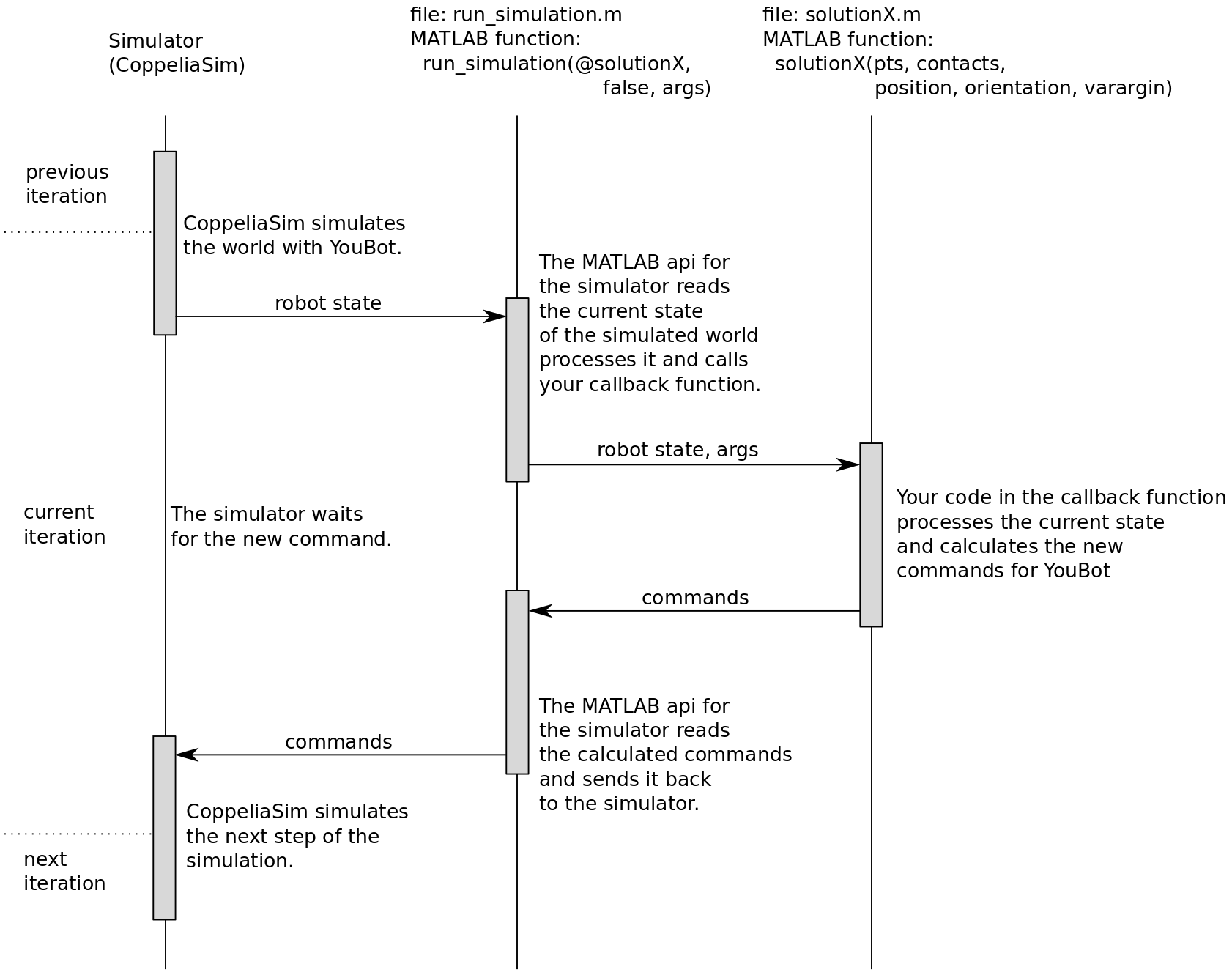
You can control a robot in CoppeliaSim from MATLAB using a callback function declared in a script. Such script is a matlab program that declares a callback function of the same name as the script, e.g. the callback function in the script solution0a.m is named solution0a. This callback function is called in every control loop. It processes the inputs:

• the measured pose (position and orientation) of the robot,
• LIDAR data, laser range sensor,

and produces the outputs that control the state of the robot:

• forward/backward velocity,
• left/right velocity,
• rotational velocity.

Running the examples

In order to run the already installed system please perform the following steps:

1. Run Matlab and run the Peter Corke’s Robotics, Vision & Control toolkit in the Matlab Command Window, e.g. nn Linux/Mac:

   cd emor_trs/matlab
   run('startup_robot.m');
   

2. Run CoppeliaSim simulator (e.g. in Linux, run ./coppeliaSim.sh in the CoppeliaSim directory).

To run the example program, follow the steps:

1. In CoppeliaSim, open scene emor_trs/youbot/vrep_env/exercise00.ttt using menu File -> Open Scene…
2. Run in the Matlab Command Window:

   cd emor_trs/youbot
   run_simulation(@solution0a, false, 1)
   

The function run_simulation runs the CoppeliaSim simulation and the control program for the youBot robot. The control program uses the callback function given as the first argument to run_simulation (in this case solution0a) to control the velocity of the robot. The callback function is called in each control cycle. It processes the sensors data and produces output: the linear and angular velocities of the robot.

You can run two other examples similar way, using different control callback functions:

• To run the second example, type in the Matlab console:

   run_simulation(@solution0b, false)
  

• To run the third example, type in the Matlab console:

   run_simulation(@solution0c, false)
  

Each of the callback functions solution0a, solution0b and solution0c takes the same arguments:

• pts, contacts - the data from the LIDAR sensor,
• position - the position vector of the robot. As the robot moves in the horizontal plane, only the first two coordinates are relevant (x,y),
• orientation - the orientation vector of the robot represented as Euler angles. As the robot moves in the horizontal plane, only the third coordinate is relevant (z).

The values returned by each callback function are:

• forwBackVel - linear velocity along the x axis of the robot,
• leftRightVel - linear velocity along the y axis of the robot,
• rotVel - angular velocity around the z axis of the robot,
• finish - a boolean value (true/false) that indicates the control program should be stopped.

This kind of control is possible due to the special construction of robot wheels - mecanum wheels enable to move a vehicle in (almost practically) any direction disregarding its current orientation.

Please get familiar with the functions solution0a, solution0b and solution0c declared in files solution0a.m, solution0b.m and solution0c.m respectively. Your task in all five tasks is to write your own control callback functions that realize the desired task. You can use the example callback functions as a reference.

You should pay special attention to the Finite State Machine (FSM) that manages the behaviours realized by the robot, e.g. in the solution0a callback function, the FSM has four states:

• init - the first state, when some variables are initialized. This state is executed only once,
• move_forward - the robot moves forward, with constant velocity. This state is executed until the robot reaches the desired pose,
• stop - the robot stops - the velocity is set to zero. This state is executed for some period of time,
• move_backward - the robot moves backward, with constant velocity. This state is executed until the robot reaches the desired pose,
• finish - the ending state of the control program.

The FSM enables the control system to realize complex tasks that need to execute a sequence of different behaviours, e.g. moving forward, stopping, moving backward.